Central Limit Theorem – Simplified
This article explains the Central Limit Theorem with examples in Python code.
According to Wikipedia, the Central Limit Theorem is defined as follows.
“In probability theory, the central limit theorem (CLT) establishes that, in many situations, for identically distributed independent samples, the standardized sample mean tends towards the standard normal distribution even if the original variables themselves are not normally distributed.”
Let’s try to decipher what the above definition means in simple terms. Suppose we draw some samples from a distribution that is not a normal (gaussian) distribution, take the mean of the samples thus drawn, and record the mean. We do this for many number of times. Now, when we plot the histogram of the recorded means, we see that the means are normally distributed.
Here are some examples. In the first example, we will see that the means of the samples drawn from the uniform distribution are normally (gaussian) distributed.
Example 1

In the above code, we are drawing n_samples number of samples (line 12) from a uniform distribution, computing the mean of the samples drawn (line 14), and collecting the mean in a list (line 16). We are performing the aforementioned for num_runs number of times (line 10). After the above code executes, we get a list of the mean values of the samples.
To get a better sense of what is going on, let’s look at some example outputs of the parts where we draw samples and get the mean.

The above output is an example of output we get when we randomly draw 10 samples from a uniform distribution, and the mean of the samples is shown below.

As mentioned earlier, these means are collected in a list. Let’s take a look at the first few mean values in the list produced by the code in figure 1.

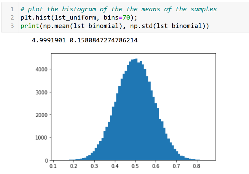
Now, when we plot the histogram of the means in the list, we get a nice bell-shaped distribution, which of course is the normal (gaussian) distribution, as shown below.

We saw that although the samples were drawn from a uniform distribution (non-gaussian), the means of the samples drawn tended towards the normal distribution. This is the Central Limit Theorem.
Example 2
Let’s see if this works for another non-gaussian distribution, such as the binomial distribution.

In the above code, we are drawing samples from the binomial distribution (line 11), which is akin to performing n_trials number of trials (e.g. flipping a coin n_trials times), and counting the number of heads we get, where the probability of getting a head is p_success, and this is repeated for n_observations times. Then we get the mean of the occurrences of head (line 13), and collect the mean values in a list (line 15). The aforementioned is repeated for num_runs times.
After the above code has executed, we will have a list of the mean values of the samples sampled from the binomial distribution.
To understand better, let’s look at the samples drawn from the binomial distribution. In the following code, we are sampling from a binomial distribution, where we perform n_trials (e.g. flipping a coin n_trials times), the probability of success (getting a head) being p_success, and we record the number of heads in each trial. We repeat this for n_observations times.

To make sense of the above output, the first number 4 in the array is the number of heads we got when flipping a coin 5 (n_trial) times in the first observation, 2 is the number of heads in the second observation and so on. We have in total 100 number of heads for 100 (n_observations) observations in the array.
When we run the above sampling for many number of times, compute the mean of the output of each run, collect the mean values, and plot a histogram of the mean values, we get a normal distribution curve, as shown below.

We saw that the mean values of the samples drawn from a binomial distribution also are normally distributed.
According to Central Limit Theorem, in most cases the mean values of the samples drawn from non-gaussian distribution tend towards a normal distribution for a large number of runs of sampling. Interestingly, even the sums (not just the means) of the samples drawn from a non-gaussian are normally distributed.